Circular Convolution Matlab Code Program (DSP)

Let us quickly go through Circular Convolution Matlab Code and go through the topic in detail after the article:

We have tried providing multiple codes for Circular Convolution MatLab Code:

Kindly go through the entire article:

Step 1: Start
Step 2: Read the first sequence
Step 3: Read the second sequence
Step 4: Find the length of the first sequence
Step 5: Find the length of the second sequence
Step 6: Perform circular convolution MatLab for both the sequences using inbuilt function
Step 7: Plot the axis graph for sequence
Step 8: Display the output sequence
Step 9: Stop

Matlab Code for Circular Convolution 

Code 1

clc;
close all;
clear all;
x1=input('Enter the first sequence :
');
x2=input('Enter the second sequence
: ');
N1=length(x1);
N2=length(x2);
N=max(N1,N2);
 
if(N2>N1)
x4=[x1,zeros(1,N-N1)];
x5=x2;
elseif(N2==N1)
        x4=x1;
        x5=x2;
else
x4=x1;
x5=[x2,zeros(1,N-N2)];
end
 
x3=zeros(1,N);
for m=0:N-1
x3(m+1)=0;
for n=0:N-1
        j=mod(m-n,N);
        x3(m+1)=x3(m+1)+x4(n+1).*x5(j+1);
end
end
 
subplot(4,1,1)
stem(x1);
title('First Input Sequence');
xlabel('Samples');
ylabel('Amplitude');
subplot(4,1,2)
stem(x2);
title('Second Input Sequence');
xlabel('Samples');
ylabel('Amplitude');
subplot(4,1,3)
stem(x3);
title('Circular Convolution Using
Modulo Operator');
xlabel('Samples');
ylabel('Amplitude');
 
%In built function
y=cconv(x1,x2,N);
subplot(4,1,4)
stem(y);
title('Circular Convolution using
Inbuilt Function');
xlabel('Samples');
ylabel('Amplitude');

If length (N1=N2) then no changes to the sequence.

elseif(N2==N1) 

x4=x1; 

 x5=x2;

and if length (N1>N2) then padding the other sequence with zeros.

x5=[x2,zeros(1,N-N2)];

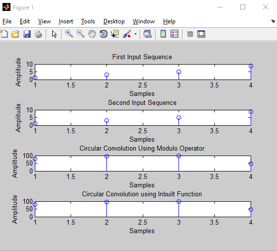
Now let’s plot the curve of the input sequences and the output of matlab code for circular convolution

subplot(4,1,1) stem(x1); 

title('First Input Sequence');

xlabel('Samples'); 

ylabel('Amplitude');

 subplot(4,1,2) stem(x2); 

title('Second Input Sequence'); 

xlabel('Samples'); 

ylabel('Amplitude'); 

subplot(4,1,3) 

stem(x3); 

title('Circular Convolution Using Modulo Operator'); 

xlabel('Samples'); 

ylabel('Amplitude');

After plotting all the axis of the graph we will be look using the inbuilt circular convolution MatLab function for performing the code.

y=cconv(x1,x2,N);

rest all lines after this are to plot the output curve we get after using the inbuilt circular convolution function in MatLab.

%In built function y=cconv(x1,x2,N); 

subplot(4,1,4)

 stem(y); 

title('Circular Convolution using Inbuilt Function'); 

xlabel('Samples'); 

ylabel('Amplitude');

Go to top

If you are looking for Linear Convolution Matlab code check it out here:

Linear Convolution Program Using Matlab

Go to top

Here is the Output

Code 2:

x = input(‘enter a sequence’);

h = input(‘enter another sequence’);

n1=length(x);

n2 = length(h);

n = max(n1,n2);

a=1:n;

x = [x,zeros(1,n-n1)];

h = [h,zeros(1,n-n2)];

y = zeros(1,n);

for i =0:n-1

for j = 0:n-1

k = mod((i-j),n);

y(i+1) = y(i+1) + x(j+1)*h(k+1);

end

end

stem(a,y)

Output:

Code 3:

MATLAB code
x1=input('Enter the sequence x1(n)=');
x2=input('Enter the sequence x2(n)=');
N=length(x1)+ length(x2)-1;
X1=fft(x1,N);
X2=fft(x2,N);
Y=X1.*X2;
y=ifft(Y);
% y is the linear convolution of x1(n) and x2(n)
disp('Linear convolution of x1(n) and x2(n) is:');
disp(y)

Circular Convolution without using inbuilt function cconv(x,y,n)

It is used to convolve 2 different discrete Fourier transforms.

It is way to fast for long sequences than linear convolutions

Code 4

Enter x(n):
[1 2 2 1]
Enter h(n):
[1 2 3 1]
x(n) is:
1 2 2 1

h(n) is:
1 2 3 1

Y(n) is:
11 9 10 12

Thus results can be achieved Circular convolution without using cconv(x,y,n)

What is Modulo-n circular convolution?

a = [1 2 -1 1];
b = [1 1 2 1 2 2 1 1];

c = cconv(a,b);            % Circular convolution
cref = conv(a,b);          % Linear convolution

dif = norm(c-cref)

For more examples visit Mathworks

What is Circular Convolution:

Circular convolution also known as cyclic convolution to two functions which are aperiodic in nature occurs when one of them is convolved in the normal way with a periodic summation of other function.

A similar situation can be observed can be expressed in terms of a periodic summation of both functions, if the infinite integration interval is reduced to just one period. This situation arises in Discrete-Time Fourier Transform(DTFT) and is called periodic convolution.

Let us consider x to be a function with a defined periodic summation, x_T, where:

If h is any other function for which the convolution x_T * h (Multiply) exists, then the convolution x_T ∗ h is periodic and equal to:

where t_o is an arbitrary parameter and h_T is a periodic summation of h.

The second integral is called the periodic convolution of functions x_T and h_T & is normalized by 1/T.

When x_T is expressed as the periodic summation of another function, x, the same operation may also be referred to as a circular convolution of functions h and x.